GRIP: testing which gene relationships survive representation changes

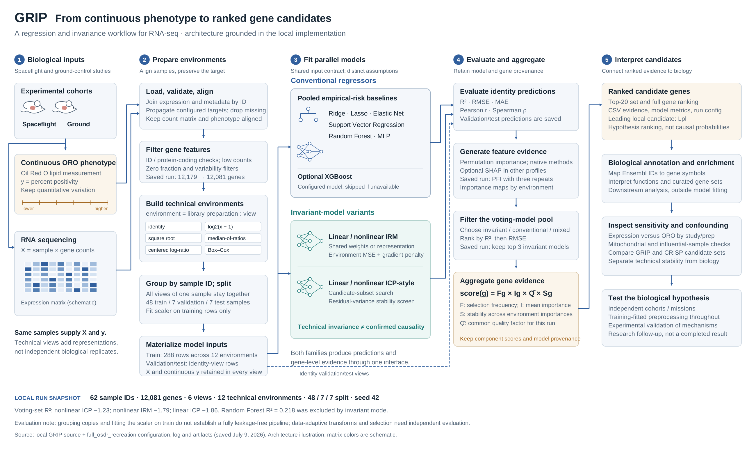
I proposed GRIP to investigate gene–phenotype relationships that remain useful across technical representations of RNA-sequencing data. The current framework combines continuous regression, transformation-based environments, invariant model variants, and ensemble gene scoring. My central question is whether a candidate remains compelling when the representation that made it look important changes.

The local Oil Red O reconstruction contains 62 sample IDs and 12,081 retained expression features. Its target measures liver lipid accumulation. This is a small-sample, high-dimensional problem: a model has many more potential explanatory variables than independent observations.

GRIP pipeline from continuous biological measurements through technical environments, parallel regressors, model filtering and gene scoring to biological interpretation — The complete GRIP workflow, drawn from the local implementation and saved reconstruction. Solid arrows show the main processing flow; the dashed route carries identity-view validation/test data to evaluation. Continuous ORO values are retained. Run dimensions describe this reconstruction, and matrix colors are schematic. Open full-size figure ↗

What the implementation taught me

Additional views do not create additional biology

The saved run uses identity, log2, square-root, median-of-ratios, centered-log-ratio, and Box–Cox views. Logarithms compress large counts; median-of-ratios adjusts sample scale; centered log-ratios express abundance relative to each sample's geometric mean. Different representations expose different dependencies in a fitted model.

Crossing these six views with two library preparations produces 12 technical environments and 372 rows. Flight status is excluded from the environment label because it may carry the biology under investigation.

The split groups transformed copies by sample ID: 48 training samples become 288 training rows, with seven identity-view samples each for validation and testing. The scaler is fitted on training rows. Grouping prevents copies of one sample crossing those partitions; validating every data-adaptive preprocessing step remains a separate requirement.

Invariance needs an operational definition

The linear IRM implementation minimizes average environment MSE plus an annealed penalty on environment-specific loss gradients with respect to the shared weights:

meanₑ MSEₑ + λ(t) Σₑ ‖∇w MSEₑ‖².

This encourages solutions that are simultaneously stationary across environments. The nonlinear variant introduces a learned representation before the prediction head.

The v1 linear ICP-style implementation instead screens genes by pooled absolute correlation, searches subsets, and fits separate regressions within environments. A Bartlett test checks residual-variance equality. Retaining a subset after that test is a limited stability screen: failing to reject unequal variance does not establish identical residual distributions or biological causality. The implementation uses a largest-accepted-subset strategy, so I treat it as an ICP-style approximation rather than assume the guarantees of canonical ICP.

Make the ranking traceable to its components

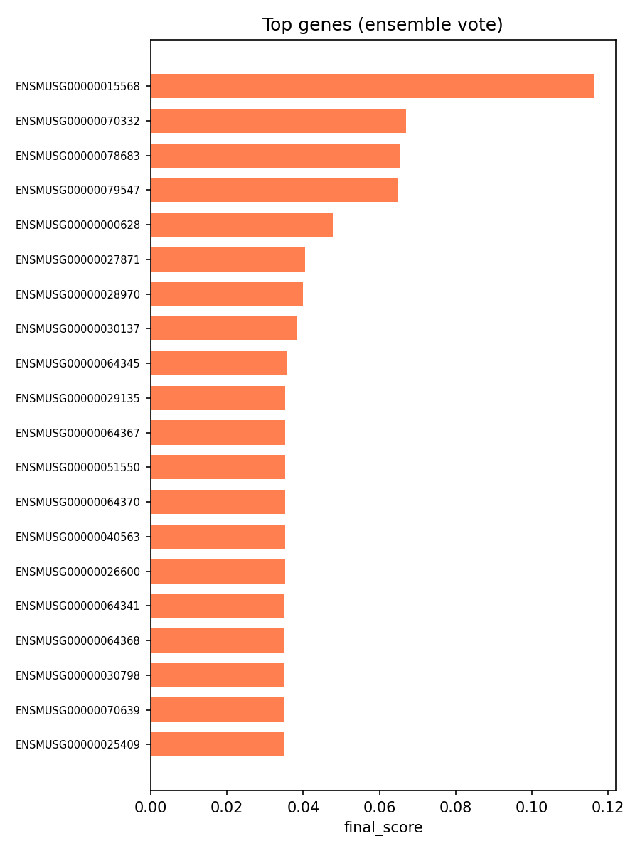
GRIP scores each gene as F_g × I_g × Q̄ × S_g: selection frequency, mean importance, mean model quality, and environment stability. Within each model, stability is clip(1 − σ/(μ + ε), 0, 1) across environment importances, then averaged across models. In this implementation, Q̄ is common to all genes; it changes score scale rather than their relative ordering. Frequency, importance, and stability determine that ordering.

Top-20 gene scores from the saved local GRIP reconstruction — The run's original ensemble-vote output. ENSMUSG00000015568, annotated as Lpl in the biological report, ranks first. These scores summarize model evidence; they are not probabilities of causality. Open full-size figure ↗

Reading the result without hiding the tradeoff

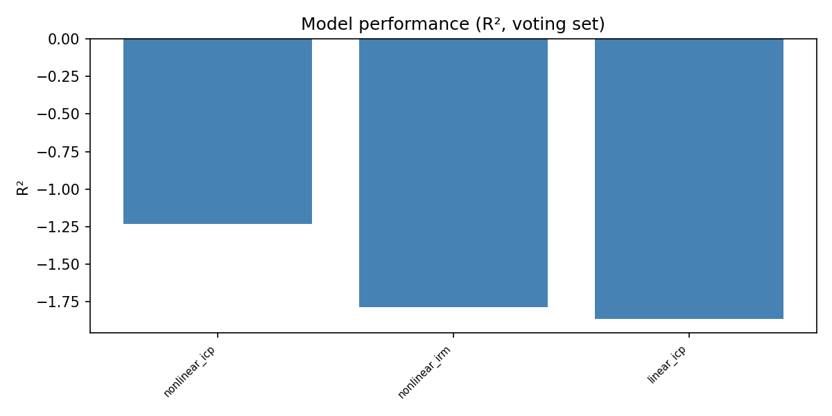
Strict invariant mode retains nonlinear ICP, nonlinear IRM, and linear ICP, with R² values of approximately −1.23, −1.79, and −1.86. A Random Forest reaches approximately 0.218 but is excluded by that mode's eligibility rule. Ranking the best eligible models does not impose an absolute performance floor.

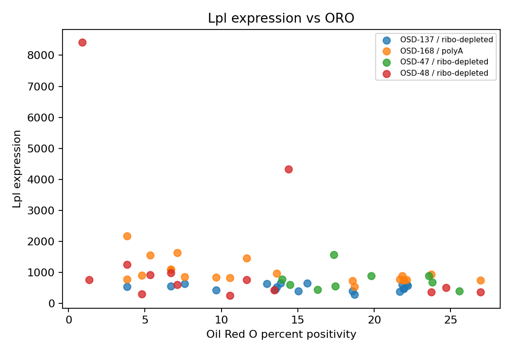
Performance of the three models retained for voting — Original local voting-set plot. All three scores are negative: each model's squared error exceeds the mean-of-evaluation-targets reference used by R². The Random Forest is outside this plotted voting set. Open full-size figure ↗

The leading candidate also needs examination at sample level. The saved Lpl-versus-ORO plot shows study/preparation groups and conspicuous high-expression points. I would test their influence before interpreting the ensemble rank as a robust biological relationship.

Lpl expression versus Oil Red O positivity, grouped by study and library preparation — Original local biological diagnostic. Group structure and high-expression observations motivate sensitivity analyses; the plot does not by itself establish a consistent within-study effect. Open full-size figure ↗

My main learning is that an inference framework should expose its own assumptions. GRIP currently produces inspectable hypotheses and concrete evaluation questions. Establishing stable discovery will require sensitivity tests, preprocessing fitted within evaluation boundaries, and independent biological validation.